HotPopRobot

Artash Nath

In September 2020,  I came across the University of Toronto Aerospace Team (UTAT) while searching for communities centered around rocketry and aerospace. UTAT is an award-winning interdisciplinary team based at the University of Toronto that designs and builds drones, rockets, and satellites. It does so by bringing together passionate students from across Canada who like solving engineering and science challenges.

One of UTAT’s divisions, Space Systems was hosting several recruitment workshops that month to reach out to new students interested in joining the team. As I have always been interested in space exploration, rocketry, and artificial intelligence, and have undertaken several projects related to them, I decided to attend their workshops. It was an excellent opportunity for me to learn more about the team, the projects they are working on, and how they collaborate with other divisions within UTAT.  I learnt that UTAT Space  Systems focused on the design, development and launching of small satellites- specifically CubeSats. They had already developed and constructed a CubeSat: HERON Mk1 from scratch. This year, they were starting to design their second CubeSat mission: FINCH.

I was enthused by their projects and passion and became interested in joining the team. UTAT Space Systems has multiple subsystems, each of which work on different aspects of the CubeSat, from electronics and firmware to science and optics. Over the next few weeks, I attended workshops led by the leads of all the divisions. During the workshops, the leads explained about the different projects they would be undertaking and what skill sets they were looking for. It was a wonderful opportunity to interact with the current team members, ask them questions, and learn about specific challenges they were working on.

The Payload-Electronic Team

After exploring all the different subsystems and learning about the projects they will be undertaking during the year, I ended up joining the Payload-Electronic (Pay-Elec) system. The Pay-Elec team handled the image capturing and storage process of the camera, which would comprise the main payload of the CubeSat. There were around 12 active Pay-Elec members working on different projects within the team. Because of Covid-19 restrictions, it was not possible to meet face to face. However, every week on Saturday evening, the team members would meet in a videocall to give progress updates, ask questions, and discuss how to go forward from there. Yong Da, was the Pay-Elec team lead. He led these weekly meetings and made sure everyone knew what to work on. In addition, there were occasional smaller meetings between members working on similar projects to review each other’s work, trouble shoot and plan for upcoming weeks.

Project Goal: Image Compression

As I have been working on python for the past 5 years and have undertaken projects on mathematical and scientific data analysis, I became interested in the “Image Compression” project. Images taken from the camera aboard the CubeSat had to be transmitted to a station on earth. But there is only a small amount of time and bandwidth available to make the transmission. The goal of the image compression project was to reduce the image size as much as possible without significant loss of information. This would ensure that data received from the CubeSat could easily be reconstructed to create detailed images. I decided to join the project and was welcomed by the other team members. It was wonderful to be working with people passionate about solving space-related challenges.

Discrete Cosine Transformation Compression

My first project within the UTAT Pay-Elec team was to use Discrete Cosine Transformation (DCT) to compress sample images in python. A DCT breaks an image into discrete layers, representing its cosine components in different frequencies. Each layer represents a different cosine frequency. When these layers are added back up, they result in the original image. But each of the layers have varying importance when recreating the original image. Some of these layers may be of higher importance (or a higher weightage) in creating the image while other layers may have almost no importance (or a lower weightage). And that is where the DCT can be used to compress an image. By discarding layers having a lower weightage, the space required to store and transmit an image can be reduced significantly. The lesser the number of layers discarded (higher compression ratio), the greater the space required to store the image. Conversely, the more the number of layers discarded (smaller compression ratio), the lesser the space required to store the image. But there is a threshold limit – too smalla compression ratio (could cause significant loss of information between the original and the reconstructed image.

I needed to find that threshold value. What was the lowestcompression ratio I could apply to the image without a significant loss of information? To do this, I needed to test out the DCT compression at different ratios and determine which one worked the best.

Discrete Cosine Transformation Python Algorithm

I wrote the entire DCT Compression process from scratch in python. My code had 5 major steps:

1. Calculate 2D Discrete Cosine Transformation of the image 
2. Order the DCT Coefficients based on weightage
3. Discard bottom 50% of the layers
4. Apply an inverse Discrete Cosine Transformation to remaining layers to reconstruct the image
5. Calculate the loss between original and reconstructed image

I altered the code to work at different compression ratios. To measure how close the reconstructed image was from the original, I had to come up with a metric that would compare the two images and quantify the loss. I decided on a function that would subtract the corresponding pixel values in each image, creating an array of pixel differences. I would then take the mean of all the pixel differences, resulting in the mean pixel value difference between the original and the reconstructed images.  The lower the mean pixel value difference, the higher the quality of the reconstructed image, or lower the information loss.

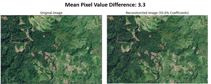
See for instance, figure 1. On the left, is the original image that is to be compressed. On the right is the image that has been reconstructed after the compressing the original one using DCT at a compression ratio of 0.5.  (i.e., half the DCT coefficients were discarded). Visually, both images look the same. I measured only a 3.3 mean pixel value difference between the two images, too little to be noticed with the human eye.

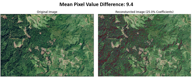
However, when I tried decreasing the compression ratio to 0.25 (see figure 2), the quality of the recreated image spiraled down. I measured a mean pixel value difference of 9.4 between the two images. It was evident that a significant amount of added noise got added in the reconstructed image that was not present in the original image.

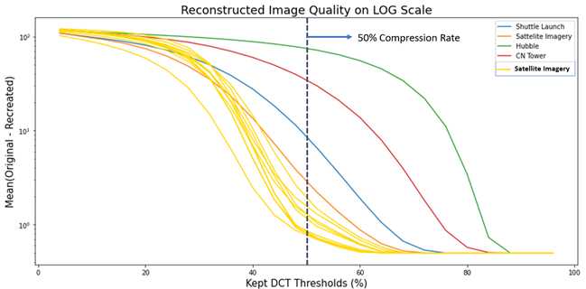
To determine the optimum threshold compression ratio, I took a sample of 10 satellite images, and 3 additional random images. I graphed the DCT Threshold Percentage (compression ratio x 100) versus the mean pixel value difference of the reconstructed image on a log scale. See Figure 3.

I found that for all sample satellite images, the mean pixel value difference rapidly increased after the compression ratio dropped below 0.5 (see figure 3). For some of the other images such as the iconic Hubble Deep Field image from the Hubble Space Telescope (figure 4), the mean pixel value difference (depicted in green line) increased dramatically after a compression ratio of just 0.9. (i.e., after discarding only 10% of the DCT coefficient layers). The entire code for this project is available at my GitHub: https://github.com/Artash-N/UTAT-JPG2DCT

Discrete Wavelet Transformation Compression

While DCT Compression was a good start – it allowed the compression of satellite imagery by up to 50% – it was not enough. The disadvantage of DCT is that as it breaks the image into its cosine components, it does not work well for images that have repeated sharp contrasts or abrupt distinct features. For instance, the iconic Hubble Deep Field image (figure 4) has multiple bright spots (stars and galaxies) against a dark background.  DCT does a poor job in compressing it.

Using DCT Compression, the lowest compression ratio that could be applied to the Hubble Deep Field image without significant loss of information was 0.9. This would not yield a significant reduction in image size needed for satellite imagery transmission.

In January 2021, I started working on a relatively new type of compression: Discrete Wavelet Transform (DWT) Compression. DWT is like DCT, in the way that it breaks down an image into coefficients in the frequency space. But there are two major differences between DCT and DWT.

First, DWT can provide the time and frequency information of a signal simultaneously, while DCT only provides the amplitude-frequency representation of the signal. Thus, DWT can analyze non-stationary signals or signals whose frequency response varies in time, while DCT only analyze stationary signals.

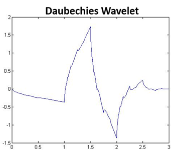
Second, DWT is not limited to breaking an image into different frequencies of the cosine signal. Instead, it can break an image into a wide variety of wavelets. A wavelet is a wave-like oscillation with an amplitude that begins at zero, increases, and then decreases back to zero. Because the DCT is limited to the cosine wave, it only works optimally for data with smoother curves and softer contrasts. However, using wavelet coefficients allow the compression of much higher frequency data and images with more contrasting features, such as the Hubble Deep Field image.  Furthermore, wavelet transformations of data result in large number of zero or near zero values, creating more room for compression (see figure 5).

Once again, I turned to python to implement the DWT compression. There were 5 steps in this program, like the DCT compression, except it involved calculating the DWT of the image instead of DCT. In DWT, we introduce a parameter called the wavelet decomposition level. The higher the decomposition level, the more the number of near-zero values in the resulting wavelet, and greater the room for compression of these images.

As shown in the histogram (figure 6) 30% of the DWT coefficients for the Hubble Deep Field image are 0-values.  Furthermore, over 90% of the coefficient values are below 10. Unfortunately, increasing the decomposition level also creates a handful of wavelet coefficients that are of extremely high magnitude, which take up a lot more storage space than smaller numbers.

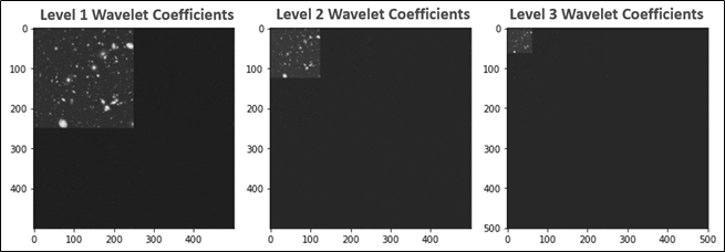
As shown in figure 7 as the decomposition level increases the image is squished towards the top left of the image, leaving near-zero values in the remaining part of the image.

I started out by testing my DWT Compression program with Level 1 compression as a baseline.

On the left is the original image. On the right is the image reconstructed after a 50% DWT compression. There is no visible difference between the original and reconstructed image and the mean pixel difference is only 1.6. In comparison, compressing this same image with DCT compression at the same decomposition level yielded a mean pixel difference of about 100 which corresponds to significant noise. It was clear that DWT turned out to be the better compression mechanism in this case.

To better understand how decomposition level affected the mean pixel value difference, I ran a function that calculated the mean pixel value difference for this image from decomposition level 1 to level 20.

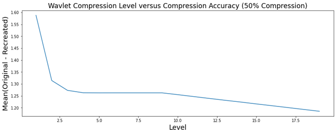
As shown in figure 9, the mean pixel difference steadily decreases as the DWT decomposition level increased. The maximum DWT level is 1000. I was curious to know how far we could keep increasing the DWT levels to bring about a decrease in the mean pixel value difference.

I plotted a similar diagram, but from level 1 to level 1000 (figure 10).

Surprisingly, after passing approximately level 200, the mean pixel difference dropped down to nearly zero. Unfortunately, the wavelet coefficients of DWT compression at level 200 contained values of up to 4.5e+61. Values this high were simply not feasible to store and defeated the purpose of compressing the image to use up as little memory as possible. After discussion with the lead of Payload-Electrical, I decided that level 100 DWT compression would be the most optimal. It would have the advantage of the increased accuracy of higher-level wavelet compression and balance out the disadvantage of extremely high values of higher-level wavelet compression.

To understand what the maximum compression ratio I could achieve with level 100 compression, I plotted the compression ratio from 0 to 1, versus the mean pixel value difference for level 100 compression.

If we consider a mean pixel value difference of 2 (equivalent to a 98.4% similarity between all the pixels of the images) to be the highest we can achieve without losing significant information, then the highest compression ratio possible using level 100 wavelet compression is about 0.2.

The full code, along with additional diagrams are available on my GitHub repo for this project: https://github.com/Artash-N/DWT-IMAGE-COMPRESSION

Conclusion

In conclusion, while DCT compression is simpler and faster, it performs poorly on high contrasting images like the Hubble Deep Field image. Level 100 DWT compression achieved a much better image compression accuracy than DCT compression on both normal and high contrasting images. With level 100 DWT compression, I was able to compress an image with a compression ratio of 0.2 without significant loss of information.